Introduction to statistical indicators for classification problems: confusion matrix, recall, false positive rate, AUROC
Abbreviation
Area Under the Curve (AUC)
Area Under the Receiver Operating Characteristic Curve (AUROC)
In many cases, AUC is used to refer to AUROC, which is not always a good practice. As Marc Claesen has pointed out, AUC can be ambiguous since it might refer to any curve, whereas AUROC is more specific and clear.
Understanding AUROC
AUROC has several equivalent interpretations:
The probability that a randomly selected positive instance is ranked higher than a randomly selected negative one.
The expected proportion of positive instances that are ranked before randomly chosen negative instances.
The expected true positive rate when the ranking is placed before a randomly drawn negative sample.
The expected ratio of negative samples ranked after a randomly drawn positive sample.
The expected false positive rate when the ranking is placed after a randomly drawn positive sample.
For a deeper understanding, you can check this detailed derivation on Stack Exchange: How to derive the probabilistic interpretation of AUROC.
Calculating AUROC
To understand how AUROC works, we first need to look at a binary classification model, such as logistic regression. Before discussing the ROC curve, it’s important to grasp the concept of the confusion matrix. A binary classifier can result in four outcomes:
Predicting 0 when the actual value is 0 — known as True Negative (TN), meaning the model correctly identifies a negative instance. For example, antivirus software correctly identifies a harmless file as safe.
Predicting 0 when the actual value is 1 — known as False Negative (FN), where the model fails to detect a positive instance. For example, an antivirus misses a real virus.
Predicting 1 when the actual value is 0 — known as False Positive (FP), where the model incorrectly labels a negative instance as positive. For example, an antivirus flags a harmless file as a virus.
Predicting 1 when the actual value is 1 — known as True Positive (TP), where the model correctly identifies a positive instance. For example, an antivirus correctly detects a virus.
With these four values, we can construct a confusion matrix, which helps evaluate the performance of our model.
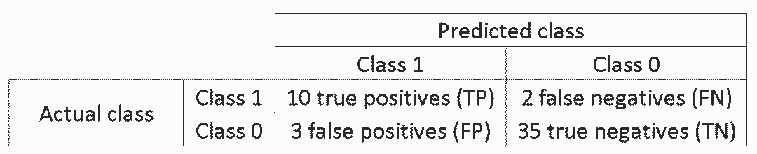
In the example above, out of 50 data points, 45 were correctly classified, and 5 were misclassified.
When comparing different models, it's often helpful to use a single metric rather than multiple ones. Two key metrics derived from the confusion matrix are:
True Positive Rate (TPR), also known as sensitivity or recall, is calculated as TP / (TP + FN). It measures the proportion of actual positives that are correctly identified. The higher the TPR, the fewer positives are missed.
False Positive Rate (FPR), also known as the fall-out, is calculated as FP / (FP + TN). It measures the proportion of actual negatives that are incorrectly identified as positives. The higher the FPR, the more negatives are misclassified.
To combine TPR and FPR into a single measure, we calculate them across various decision thresholds (e.g., 0.00, 0.01, ..., 1.00). Plotting FPR on the x-axis and TPR on the y-axis gives us the ROC curve. The area under this curve is called AUROC.
The image below illustrates the AUROC curve:
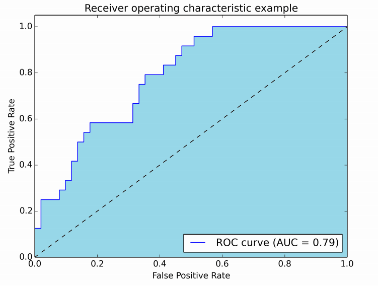
In the figure, the blue area represents the AUROC. The diagonal dashed line corresponds to a random classifier with an AUROC of 0.5, which serves as a baseline for comparison.
If you want to experiment with AUROC yourself, here are some resources:
Python: Scikit-learn ROC Example
MATLAB: MathWorks Documentation
Dongguan Jili Electronic Technology Co., Ltd. , https://www.jlglassoca.com